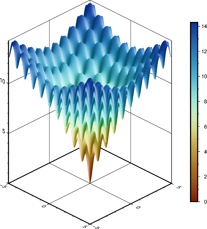
Plotting a surface

The pygmt.Figure.grdview method can plot 3-D surfaces with surftype="s". Here, we supply the data as an xarray.DataArray with the coordinate vectors x and y defined. Note that the perspective parameter here controls the azimuth and elevation angle of the view. We provide a list of two arguments to frame - the first argument specifies the \(x\)- and \(y\)-axes frame attributes and the second argument, prepended with "z", specifies the \(z\)-axis frame attributes. Specifying the same scale for the projection and zscale parameters ensures equal axis scaling. The shading parameter specifies illumination; here we choose an azimuth of 45° with shading="+a45".

import numpy as np
import pygmt
import xarray as xr


# Define an interesting function of two variables, see:
# https://en.wikipedia.org/wiki/Ackley_function
def ackley(x, y):
    """
    Ackley function.
    """
    return (
        -20 * np.exp(-0.2 * np.sqrt(0.5 * (x**2 + y**2)))
        - np.exp(0.5 * (np.cos(2 * np.pi * x) + np.cos(2 * np.pi * y)))
        + np.exp(1)
        + 20
    )


# Create gridded data
INC = 0.05
x = np.arange(-5, 5 + INC, INC)
y = np.arange(-5, 5 + INC, INC)
data = xr.DataArray(ackley(*np.meshgrid(x, y)), coords=(x, y))

fig = pygmt.Figure()

# Plot grid as a 3-D surface
SCALE = 0.5  # in centimeters
fig.grdview(
    data,
    # Set annotations and gridlines in steps of five, and
    # tick marks in steps of one
    frame=["a5f1g5", "za5f1g5"],
    projection=f"x{SCALE}c",
    zscale=f"{SCALE}c",
    surftype="s",
    cmap="roma",
    perspective=[135, 30],  # Azimuth southeast (135°), at elevation 30°
    shading="+a45",
)

# Add colorbar for gridded data
fig.colorbar(
    frame="a2f1",  # Set annotations in steps of two, tick marks in steps of one
    position="JMR",  # Place colorbar in the Middle Right (MR) corner
)

fig.show()